Finding the Electric Field from the Electric Potential (difference)

I’m way behind on this one. My plan was to write up something when this question came up in the summer section of algebra-based physics. It was a great question and deserved a full answer. Also, I wanted to make this a tutorial on trinket.io—but maybe I will do that after I write about it here.

So, here’s how it goes. We start off the semester calculating the electric field due to a point charge and then due to multiple point charges (you know—like 2). After that we get into the electric potential difference. Both the potential and the field follow the superposition principle. If you calculate the value due to two charges individually, you can add these together to get the total field or potential.

But there is a big difference. The electric potential difference is a scalar value where as the electric field is a vector. That means that when using the superposition with electric fields, you have to add vectors. Students would prefer to just add scalars—I’m mean, that seems obvious. Does that means that you could just find the electric potential difference for some set of point charges and then use that potential to find the electric field? Yup. You can. And we will.

Let me start with the definition of the electric potential difference. Since it’s really just based on the work done by a conservative force (the electric field), this looks a lot like the definition of work.

$\Delta V = -\int_a^b \vec{E}\cdot d\vec{r}$

Yes, that’s an integral. Yes, I know I said this was for an algebra-based course. But you can’t deny the truth. The “a” and “b” on the limits of integration are the starting and ending points—because remember, it’s really an integral. Also, the “dr” is in the direction of the path from a to b. It doesn’t technically have to be a straight line.

What about an algebra-based course? Really, there are only two options. The most common approach gives the following two equations for electric potential.

$V = k\frac{q}{r}$

$\Delta V = -E\Delta r \cos \theta$

The first expression is the electric potential of a point charge with respect to infinity (so the starting point for the integral is an infinite distance away). The second expression is the change in electric potential due to a constant electric field when there is an angle between the field and the displacement.

Oh wait! I forgot to list the value of k. This is the Coulomb constant.

$k = 9\times 10^9\text{ N*m}^2\text{/C}^2$

Students can understand the second expression because it’s pretty much the same as the definition of work (for a constant force). The first equation is mostly magic. The one way you can show students where it comes from is to do a numerical calculation of the electric potential difference since they can’t integrate. Did I write about that before? I feel like I did.

Ok, that’s a good start. Now for a problem.

Electric potential due to two point charges

Suppose I have two charges that are both located on the x-axis. Charge 1 is at the origin with a charge of 6 nC. Charge 2 is at x = 0.02 meters with a charge of -2 nC. Here’s a diagram—just for fun.

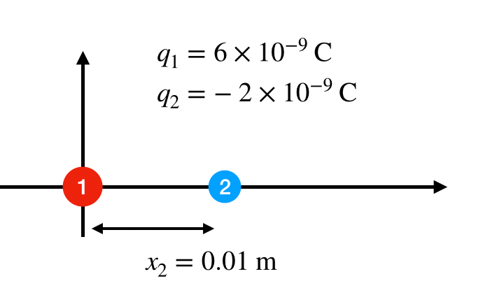
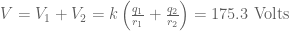
Let’s start off with the electric potential—as a warm up. What is the value of the electric potential (with respect to infinity) at the location of x = 0.02 meters? Using the equation above for the electric potential due to a point charge, I need to find the potential due to point 1 and then the potential due to point 2—then just add them together (superposition).

First for point 1.

$r_1 = 0.02\text{ m} - 0\text{ m} = 0.02$

$V_1 = k\frac{q_1}{r_1}$

Now for point 2.

$r_2 = 0.02\text{ m} - 0.01\text{ m} = 0.01$

$V_2 = k\frac{q_2}{r_2}$

This gives a total electric potential:

$V = V_1 + V_2 = k\left(\frac{q_1}{r_1} + \frac{q_2}{r_2}\right) = 175.3\text{ Volts}$

Finding the Electric Field

Now to find the electric field at that same point. I don’t know how to say this in a nice way, so I will just say it. Since the electric potential is calculated based on an integral of the electric field, the electric field would be an anti-integral. Yes, this means it’s a derivative. But wait! The electric field is a vector and the electric potential is a scalar? How do you get a vector from a scalar? Well, in short—it looks like this.

$\vec{E} =-\nabla V$

That upside delta symbol is the del operator. It also looks like this:

$\nabla V = \frac{\partial V}{\partial x}\hat{x} + \frac{\partial V}{\partial y}\hat{y} + \frac{\partial V}{\partial z}\hat{z}$

Yes, those are partial derivatives. Sorry about that. But you do get a vector in the end. But how can we do this without taking a derivative? The answer is a numerical derivative. Here’s how it works.

Suppose I find the electric potential at three points on the x-axis. The first point is where I want to calculate the electric field. I will call this $x_0$ . The next point is going to be a little bit higher on the x-axis at a location of $x_0+dx$ . The final point will be a little bit lower on the x-axis at $x_0-dx$ . Maybe this diagram will help.

When I take these two end points (not the middle one), I can find the slope. That means the x-component of the electric field will be:

$E_x(x_0) = -\frac{V(x_0+dx)-V(x_0-dx)}{2dx}$

Let’s do this. I’m going to find the x-component of the electric field at that same location (x = 0.02 meters). I don’t want to write it out, so I’m going to do it in python. Here is the link (I wish I could just embed the trinket right into this blog post).

Umm..wow. It worked. Notice that I printed the electric field twice. The first one is from the slope and the second one is by just using the superposition for the electric field. Yes, I knew it SHOULD work—but it actually worked. I’m excited.

Also, just for fun—here is a plot of the electric potential as a function of x. The negative of this slope should give you the x-component of the electric field.

Here you can see something useful. Where on this plot is the electric field (the x-component) equal to zero? Answer: it’s where the slope of this plot is zero (yes, it’s there). Remember, just because the electric field is zero that doesn’t mean the electric potential is zero.

Homework

How about this? See if you can find the electric field due to these two charges at a location y = 0.01 and x = 0.0 meters. This is right on the y-axis, but now the electric field clearly has both an x and a y-component. That means you are going to have to do this twice.

Rhett Allain's Stuff

Confusion is the sweat of learning

Finding the Electric Field from the Electric Potential (difference)

Leave a Reply Cancel reply

Share this:

Like this:

Related

Leave a Reply Cancel reply